- Published: 2025-09-05
- Updated: 2025-09-09
- MeshLib Team
What is Iterative Closest Point?
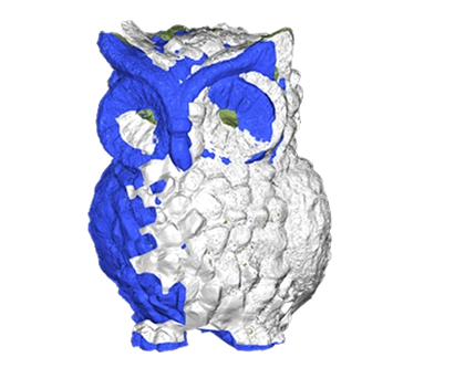
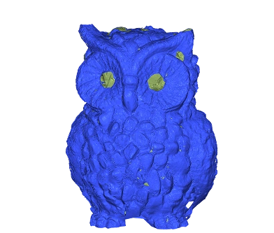
Iterative Closest Point (ICP) is, effectively, an algorithm that aligns two given 3D datasets. It takes a source object, i.e., a point cloud or a mesh, and estimates a rigid transformation, i.e., translation and rotation, that brings it into the same coordinate frame as the target object: so that their shapes match (also, in MeshLib, a non-rigid mode is also available, though it is not enabled by default and is rarely needed). This is secured by iteratively minimizing the distance between corresponding points in the two datasets.
The importance of this math algorithm is evident across:
- 3D point cloud registration, where ICP is employed for aligning scans from different viewpoints into a single model.
- Computer vision, where it is applied to object pose estimation, scene reconstruction, camera tracking, etc.
- Robotics, where it is utilized for localization and mapping, as well as aligning sensor data (e.g., from LiDAR) with existing maps.
The Iterative Closest Point Algorithm Explained
Having said this, it is self-evident that any ICP implementation might face such challenges as noise, outliers, and irregularities, whether you work with small object scans or large-scale LiDAR point clouds. For tackling this obstacles, several specialized variants have evolved:
- Point-to-Point ICP. This one aligns datasets by minimizing the Euclidean distance between corresponding points;
- Point-to-Plane ICP. Regarding this one, it focuses on reducing the perpendicular distance between source points and the tangent planes of the target;
- Combined ICP (i.e., Point-to-Point plus Point-to-Plane), finally, integrates the strengths of both Point-to-Point and Point-to-Plane methods. In actual practice, this mix is frequently employed together with outlier rejection strategies to improve robustness on noisy or incomplete datasets.
Point-to-Point ICP

Point-to-Plane ICP

Combined ICP

Notes: regardless of the variant of choice, robust and precise point cloud alignment universally depends on two additional factors. So, in any situation the best iterative closest point algorithm will be shaped by:
- Correspondence estimation, i.e., the process of identifying which points in the source dataset match points in the target. Accurate correspondences make sure that your transformation is computed from meaningful geometric relationships, instead of mismatched points;
- Convergence criteria, i.e., the rules that determine when ICP stops iterating, typically based on changes in transformation parameters, residual error, or both. Well-chosen criteria prevent premature termination or unnecessary computation. As a result, the algorithm finishes at the correct alignment.
What is noteworthy is that MeshLib allows you to rely on our ICP capabilities with outstanding control. Here is our ICP algorithm explanation in the context of MeshLib.
Support for Point Clouds and Meshes
The MeshLib library works with both unstructured point clouds and structured 3D meshes productively. Such situation of versatility makes our library a suitable pick for a wide range of applications.
Also, MeshLib can handle datasets with initial transformations already applied or dynamically adjust alignments throughout the process, all aimed at precision.
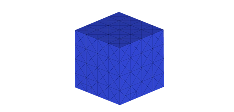
Meshes
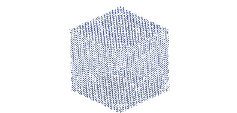
Point clouds
Transformation Calculation
MeshLib computes all the crucial transformations required for alignment:
- Rotation aligns the orientation of the source dataset with the target;
- Translation adjusts the position of the source in 3D space;
- Scaling is available for cases where the source and target datasets differ in size, boosting flexibility.
Both point-to-point and point-to-plane ICP methods are supported, upholding accuracy in various alignment scenarios.
A combination of these two techniques can be utilized, as well.
Correspondence Management
Tracking and Managing Matches
As for this one, it runs one positive Laplacian step followed by a slightly larger negative step, which cancels the volume loss while still damping noise. Think of it as two quick pushes, first out, then in, that leave the object the same size but much smoother. Though more stable than plain Laplacian, it scales poorly on extremely dense meshes.
Weighted and Filtered Matches
To secure proper dependability, the MeshLib library filters correspondences. This is accomplished by relying on similarity in surface normals and proximity. The most relevant matches are considered. Such a measure minimizes the impact of outliers or noisy data. By assigning weights to correspondences. All in all, the MeshLib library prioritizes critical areas of the dataset and ensure robustness under challenging conditions.
Iterative Refinement and Stopping Criteria
Dynamic Iterations
The MeshLib library refines alignments incrementally, minimizing misalignments at each iteration at the same time. The process continues until one of several stopping criteria get met:
- Hitting a predefined error threshold;
- Attaining the maximum number of iterations;
- Seeing no further meaningful improvements.
This reveals both efficiency and precision for final alignment.
Multiway Alignment
As for more complex workflows, the MeshLib library excels at aligning multiple datasets concurrently. Namely, we maintain global consistency across all objects. Such a capability is invaluable for tasks involving batch processing or multi-object environments, such as assembling 3D models from multiple scans.
How to Use Iterative Closest Point in MeshLib?
With MeshLib, the choice between point-to-point, point-to-plane, and the mixed approach is controlled via ICPProperties that you pass to ICP.setParams(…) before calling calculateTransformation().
Here is what happens under the hood. The ICP algorithm aligns a source dataset with a target dataset. It does so by means of a couple of transformations:
- ICP rotation. Here, the thing is to adjust the orientation of the source dataset relative to the target. This is resolved via a rotation matrix (R). The latter defines the angles of rotation around 3D axes;
- ICP translation. In this respect, we shift the source dataset’s position in 3D space. It is defined by a translation vector (T). It specifies the direction and magnitude of the shift;
- Also, as long as MeshLib is involved, the ICP scaling option is also supported. It adjusts the size of the source dataset to match the scale of the target. In our case, this manipulation is represented by a scale matrix (S), which applies scaling along axes.
ICP refines transformations iteratively. That is, it progressively minimizes misalignments between the source and target datasets. Such a flow suggests a range of key steps that get repeated over and over again, until the algorithm eventually converges:
- Correspondence identification. At the start of each iteration, the ICP algorithm identifies corresponding points between the source and target datasets. This is executed by detecting the nearest neighbour in the target dataset per each point in the source dataset;
- Correspondence filtering. Before calculating the transformation, the algorithm filters out poor matches, keeping only the most reliable correspondences for alignment;
- Transformation calculation. Once correspondences are established, the algorithm computes the optimal rotation and translation. The purpose here is to minimize the distance between the corresponding points. When scaling is enabled, the algorithm also computes a scaling factor. That promises that datasets differing in size can be properly aligned;
- Convergence and stopping criteria. Iterations continue until the algorithm converges. That means the following: any subsequent iterations will not yield significant improvements. In actual practice, ICP implementations with MeshLib rely on a combination of predefined stopping conditions. Once any of these conditions is met, the algorithm halts:
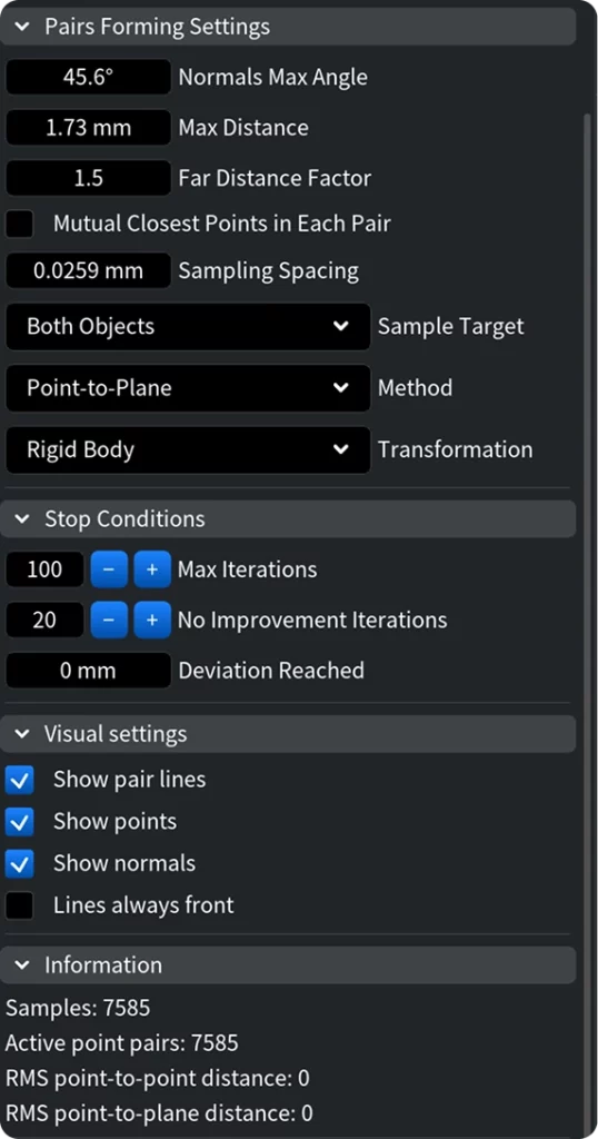
Registration tool settings in MeshInspector app
- Max number of iterations through iterLimit(int). An upper limit on iterations ensures that our process concludes even if the algorithm has yet to fully converge. This measure prevents infinite loops or excessive computation time;
- Error threshold through exitVal(float). Also, the algorithm continuously measures an error metric (based on the distance between corresponding points). If this error drops below a user-defined tolerance, it is assumed that the alignment is sufficiently refined. So, further computation might not be worth the cost;
- Deteriorating iterations count through badIterStopCount. Although ICP is aimed at reducing alignment errors, practical conditions might bring about occasional steps where the error does not improve or even slightly worsens. In case the ICP algorithm runs too many consecutive “deteriorating” iterations (i.e., those where the error does not decrease), it stops. This prevents the flow from stagnating or wasting time and resources.
Code Examples in Python & C++
When you feel preoccupied with your ICP implementation details, here are some MeshLib’s hints on how to tune the flow:
					import meshlib.mrmeshpy as mrmeshpy

# Load meshes
meshFloating = mrmeshpy.loadMesh("meshA.stl")
meshFixed = mrmeshpy.loadMesh("meshB.stl")

# Prepare ICP parameters
diagonal = meshFixed.getBoundingBox().diagonal()
icp_sampling_voxel_size = diagonal * 0.01  # To sample points from object
icp_params = mrmeshpy.ICPProperties()
icp_params.distThresholdSq = (diagonal * 0.1) ** 2  # Use points pairs with maximum distance specified
icp_params.exitVal = diagonal * 0.003  # Stop when this distance reached

# Calculate transformation
icp = mrmeshpy.ICP(meshFloating, meshFixed,
                   mrmeshpy.AffineXf3f(), mrmeshpy.AffineXf3f(),
                   icp_sampling_voxel_size)
icp.setParams(icp_params)
xf = icp.calculateTransformation()

# Transform floating mesh
meshFloating.transform(xf)

# Output information string
print(icp.getLastICPInfo())

# Save result
mrmeshpy.saveMesh(meshFloating, "meshA_icp.stl")
					#include <MRMesh/MRBox.h>
#include <MRMesh/MRICP.h>
#include <MRMesh/MRMesh.h>
#include <MRMesh/MRMeshLoad.h>
#include <MRMesh/MRMeshSave.h>

#include <iostream>

int main()
{
    // Load meshes
    auto meshFloatingRes = MR::MeshLoad::fromAnySupportedFormat( "meshA.stl" );
    if ( !meshFloatingRes.has_value() )
    {
        std::cerr << meshFloatingRes.error() << std::endl;
        return 1;
    }
    MR::Mesh& meshFloating = *meshFloatingRes;

    auto meshFixedRes = MR::MeshLoad::fromAnySupportedFormat( "meshB.stl" );
    if ( !meshFixedRes.has_value() )
    {
        std::cerr << meshFixedRes.error() << std::endl;
        return 1;
    }
    MR::Mesh& meshFixed = *meshFixedRes;

    // Prepare ICP parameters
    float diagonal = meshFixed.getBoundingBox().diagonal();
    float icpSamplingVoxelSize = diagonal * 0.01f; // To sample points from object
    MR::ICPProperties icpParams;
    icpParams.distThresholdSq = MR::sqr( diagonal * 0.1f ); // Use points pairs with maximum distance specified
    icpParams.exitVal = diagonal * 0.003f; // Stop when distance reached

    // Calculate transformation
    MR::ICP icp(
        MR::MeshOrPoints{ MR::MeshPart{ meshFloating } },
        MR::MeshOrPoints{ MR::MeshPart{ meshFixed } },
        MR::AffineXf3f(), MR::AffineXf3f(),
        icpSamplingVoxelSize );
    icp.setParams( icpParams );
    MR::AffineXf3f xf = icp.calculateTransformation();

    // Transform floating mesh
    meshFloating.transform( xf );

    // Output information string
    std::string info = icp.getStatusInfo();
    std::cerr << info << std::endl;

    // Save result
    if ( auto saveRes = MR::MeshSave::toAnySupportedFormat( meshFloating, "meshA_icp.stl" ); !saveRes )
    {
        std::cerr << saveRes.error() << std::endl;
        return 1;
    }
}
ICP Applications
When you feel preoccupied with your ICP implementation details, here are some MeshLib’s hints on how to tune the flow:
- Point-to-Point ICP will work for when you deal with raw point clouds without reliable normals and relatively sparse or noisy data, while seeking smaller pose errors;
- Point-to-Plane ICP is a match when you face dense clouds or meshes with good normals, as well as smooth and locally planar geometries, and need faster convergence near the solution;
- Combined ICP approaches are fine for heterogeneous scenes that mix edges, corners, and smooth patches, partial overlaps and moderate noise where a single metric underperforms.
Step-by-Step Instructions
-
Prepare the input data. Provide the floating and reference datasets.
Set your desired ICP parameters before starting the iterations, e.g.:
- Choose the transformation mode. Decide whether to solve for full 3D rotation and translation, translation only, or rotation around a fixed axis.
- Select the ICP method and set convergence criteria. Define the maximum number of iterations, an acceptable error threshold, and the number of consecutive non-improving iterations allowed before stopping.
- Sample points for efficiency (optional, our ICP algorithm can sample points on its own if needed, without tuning). This step, done before ICP iterations begin, reduces the number of points used in calculations to speed up processing and improve stability while preserving overall geometry.
- Run the alignment. On each iteration, the algorithm forms pairs from the sampled points and filters them, removing those that are too far apart, have significantly different surface orientations, or lie outside the region of interest. Along the way, it computes the optimal transformation, applies it to the source, and refines the alignment until one of the stopping conditions is met.
- Review the results. Check the final alignment quality, including residual error and the number of active point pairs, to confirm that the process converged as expected.
MeshLib Library – Iterative Closest Point Techniques
Video Overview
Performance
When it comes to 3D data processing, including ICP-related tasks, MeshLib is notable for the fact that our SDK delivers both high performance and precision. Our in-house benchmarks highlight up to 10× faster execution compared to alternative options.
Supported Programming Languages and Versions
Here, our users are. free to build upon us as a library for Python & C++:
- Full C++ support on all platforms without restrictions.
- Python bindings are easily available for versions 3.8 through 3.13
(with some platform-specific notes):- Windows: Python 3.8–3.13
- macOS: 3.8–3.13 (excluding 3.8 on Intel-based macOS)
- Linux: 3.8–3.13 on any manylinux_2_31+ distribution
With these bindings, you can set up and run ICP workflows in just a few lines of code, enabling rapid prototyping and integration into existing pipelines.
Our iterative closest point algorithm on Github.
What our customers say
Thomas Tong
Founder, Polyga

Gal Cohen
CTO, customed.ai
Mariusz Hermansdorfer
Head of Computational Design at Henning Larsen Architechts

HeonJae Cho, DDS, MSD, PhD
Chief Executive Officer, 3DONS INC

Ruedger Rubbert
Chief Technology Officer, Brius Technologies Inc


Start Your Journey with MeshLib
MeshLib SDK offers multiple ways to dive in — from live technical demos to full application trials and hands-on SDK access. No complicated setups or hidden steps. Just the tools you need to start building smarter, faster, and better.